Integrating CLS into Grafana and Replacing ES as Data Source
Unduh
Mode fokus
Ukuran font
Terakhir diperbarui: 2026-06-04 18:17:48
Background
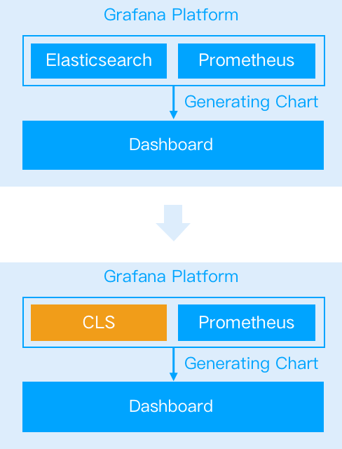
In CLS use cases, it is very common to migrate the data source from other log tools to CLS. If you use ES as the data source and Grafana as the visual monitoring tool, after you migrate the data source to CLS, various dashboard resources and Ops tools and platforms created based on Grafana will become useless. To avoid building this system again, CLS needs to be connected to Grafana to replace the ES data source.
Installing Tencent Cloud Monitor
The Tencent Cloud Monitor plugin (CLS data source) is maintained by the CLS team and has been officially signed by Grafana. You can quickly install it on the Grafana settings page.
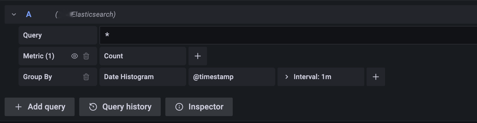
ES Data Source: The query statement page is divided into the top Query input area and the remaining auxiliary input area. You can enter Lucene statements in the Query input area to filter logs. The auxiliary input area generates DSL content by clicking and filling, which is used for data aggregation and is equivalent to CLS SQL.
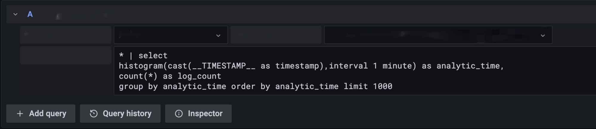
CLS Data Source: The query statement page is divided into two parts: region and log topic selection and search and analysis statement. The region and log topic selection module allows you to quickly switch log topics, while the search and analysis statement area is used to enter CLS query statements.
A CLS query statement consists of two parts: Lucene and SQL, separated by a pipe symbol "|". The Lucene part is the same as the content in the ES Query input area. In addition to standard SQL syntax, the SQL input content supports a large number of SQL functions. The SQL area content is equivalent to the auxiliary input module in the ES input area. For more information, see CLS Syntax Rules.
Directions
Counting logs
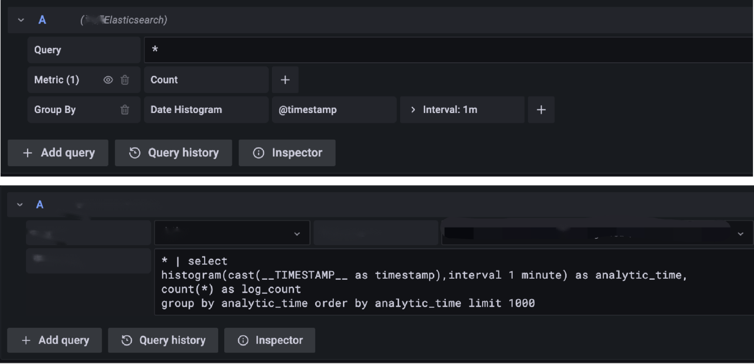
To plot the number of logs over time, select Count as the Metric and Histogram as the GroupBy in the ES data source. In CLS, you can use the Histogram function combined with the Count aggregation function in the search statement. Similarly, the usage is identical for other common aggregation functions such as Max, Min, and Distinct. You can simply replace the Count function with them.
Viewing raw logs
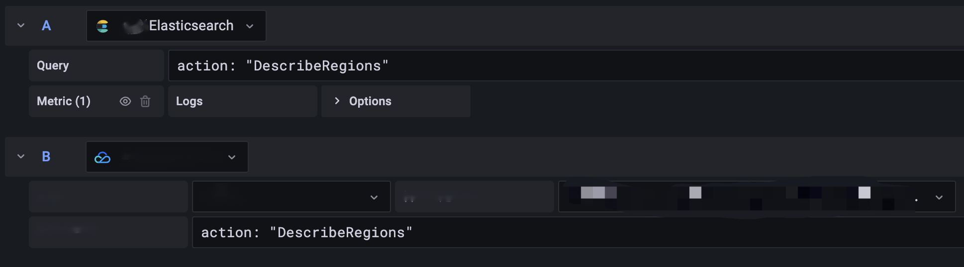
To directly view logs that meet the conditions, you need to select Logs as the Metric in the ES data source, while for CLS, you only need to enter the corresponding Lucene statement. The input statements are compared as follows:
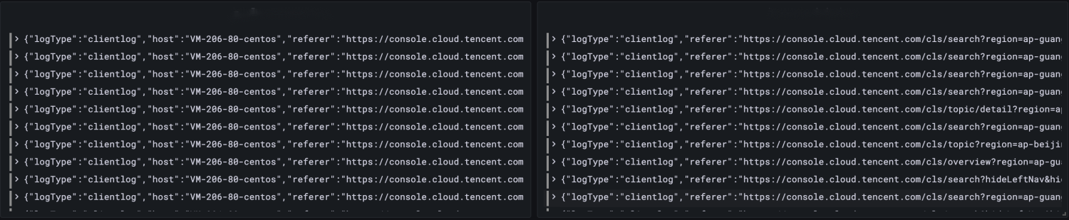
Display effect:
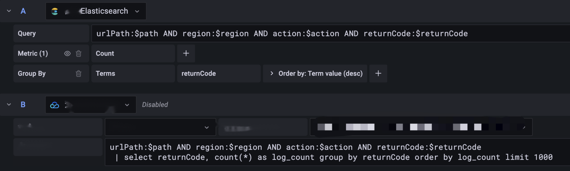
Aggregate statistics - error code proportion
You can aggregate error codes and display the numbers of logs with each error code. As can be seen here, the statement contains the
Note:
When creating a pie chart, select ValueOptions-AllValues in the chart options on the right.
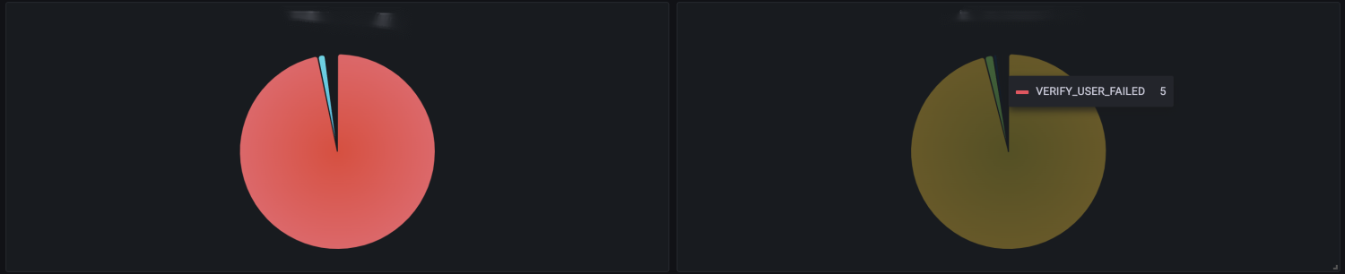
Display effect:
Aggregate statistics - changes in numbers of top five requests
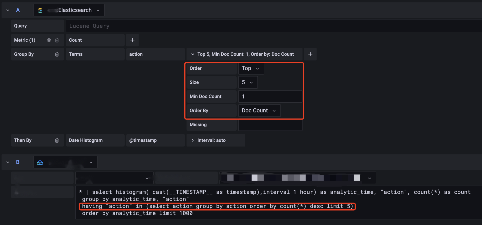
In the ES data source, the GroupBy aggregation option allows you to specify a Size value. This supports selecting the top N most frequent values for aggregation.
In the CLS data source SQL, you can implement this scenario by using a having clause with a nested subquery.
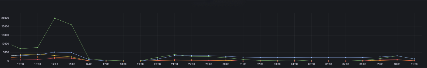
The query result shows that the chart contains five curves.
The combination of statements described above can meet the requirements of most search and analysis scenarios.
Ranged statistics of API call time
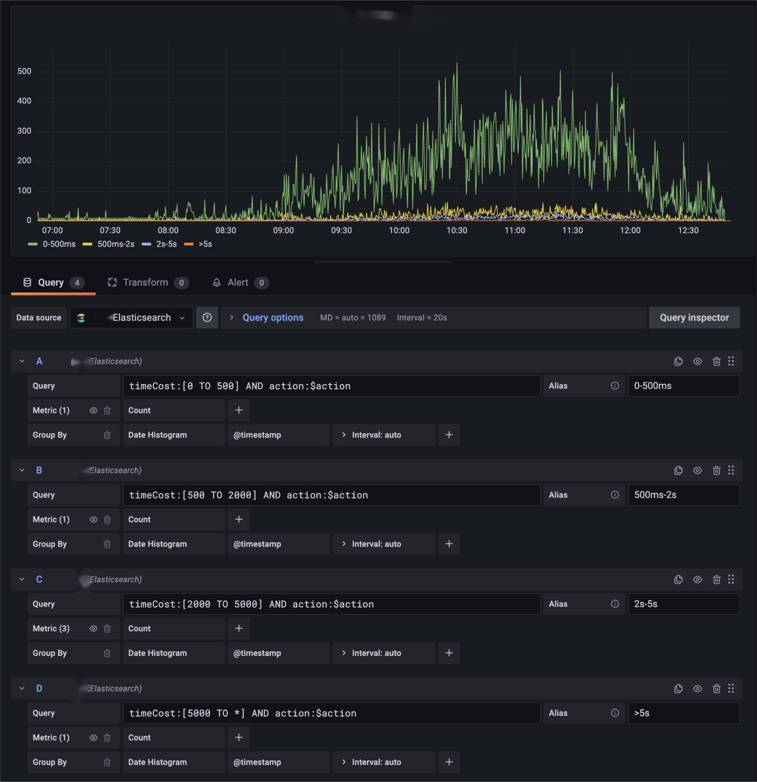
In the ES data source dashboard, there is an example with numerous configuration items but broad applicability: it plots the number of requests within a specified time range.
This example counts the number of API requests within 0-500ms, 500ms-2s, 2s-5s, and over 5 seconds.
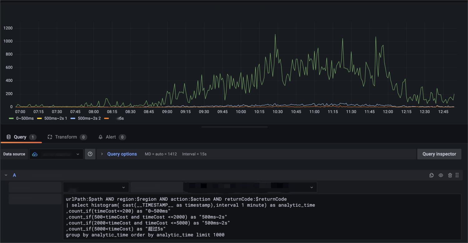
Correspondingly, when the migration to the CLS data source is performed, you can also use similar multiple statements for plotting. However, CLS has more powerful SQL capabilities, allowing you to consolidate the related statistical processing into a single SQL statement:
urlPath:$path AND region:$region ANDaction:$actionAND returnCode:$returnCode |select histogram( cast(__TIMESTAMP__ astimestamp),interval1minute)as analytic_time ,count_if(timeCost<=200)as"0~500ms",count_if(500<timeCost and timeCost <=2000)as"500ms~2s",count_if(2000<timeCost and timeCost <=5000)as"2s~5s",count_if(5000<timeCost)as"Above 5s"groupby analytic_time orderby analytic_time limit1000
For similar scenarios, we can also describe the time consumption details derived from analysis using the estimation function approx_percentile.
The Grafana variable feature is used in all of the above examples to different degrees. Grafana has diverse variable types. For constant and textbox types, they are completely the same for different data sources and don't require additional configuration for migration. This section describes how to migrate variables of query type.
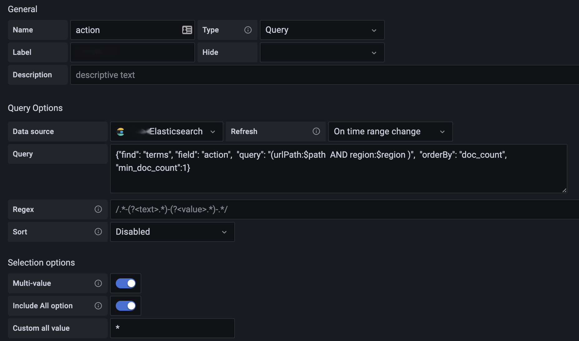
ES edition $action variable: This variable is used to display the types of APIs that appear. In the ES data source version, DSL is used for description. Semantically, it finds content that matches the query condition urlPath:$path AND region:$region, then selects the action field, and sorts the results by number of occurrences.
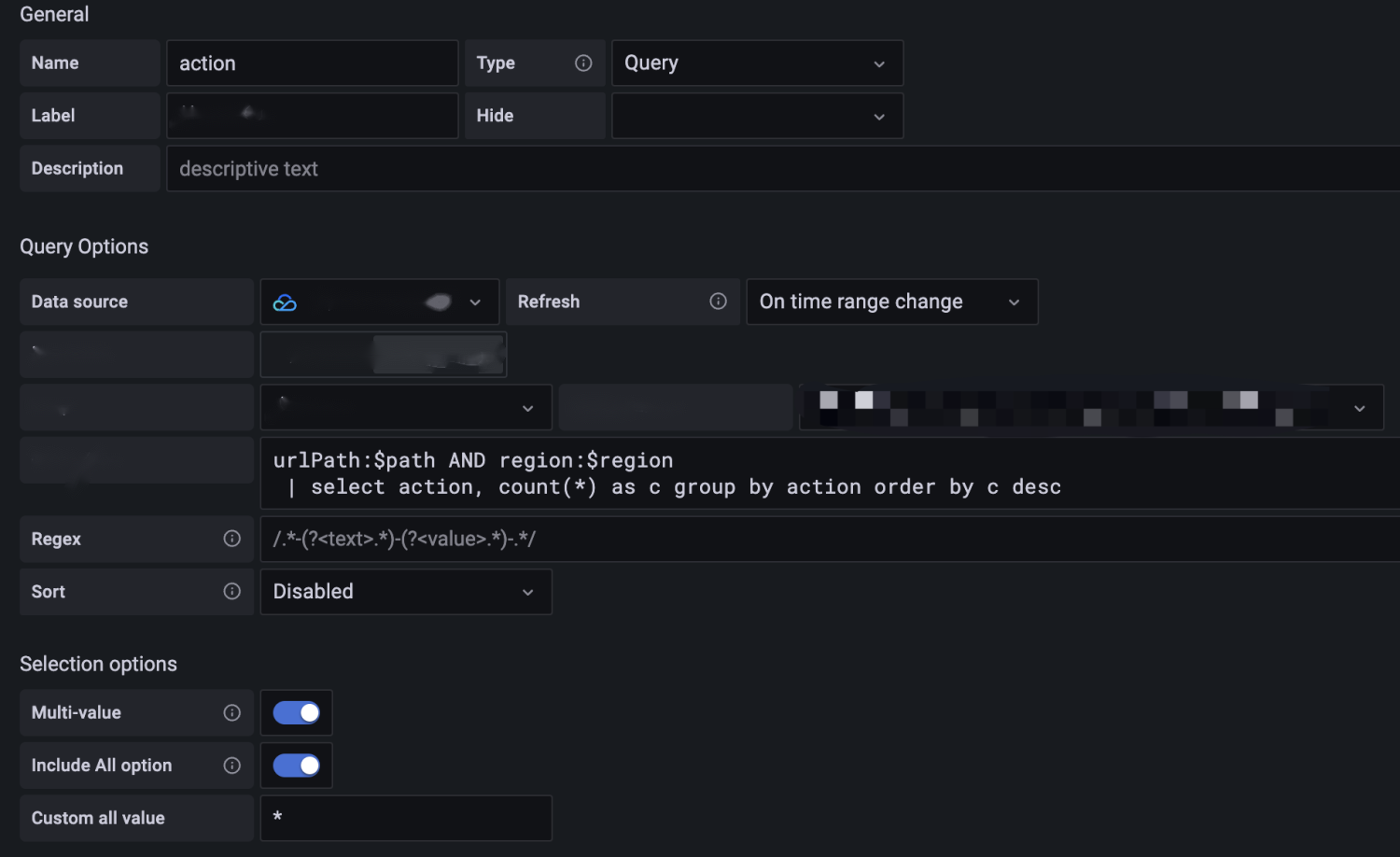
CLS edition $action variable: It provides a consistent user experience and input behavior as in chart editing. After you select CLS as the service type and choose the corresponding log topic, you can achieve the same effect by entering an SQL statement.
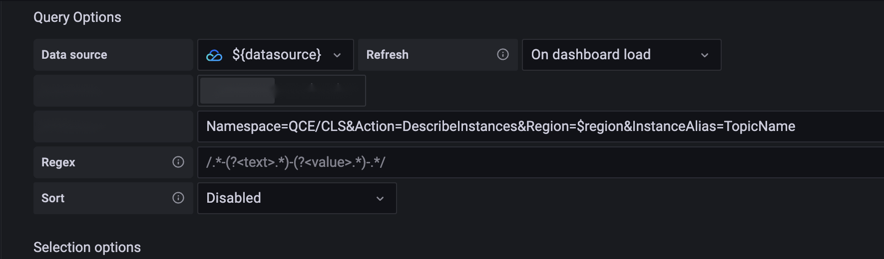
In addition to using CLS search statements for variable queries, you can also use the resource query feature of Cloud Monitor to display Tencent Cloud service resources as a list. For the feature documentation, see Cloud Monitor Data Source Template Variables. For example, you can use the following statement:
Merging data content of requests from different regions
In the original implementation, if you store all data in the same ES instance, after CLS is used, you may want to merge the content of those log tops into the same chart.
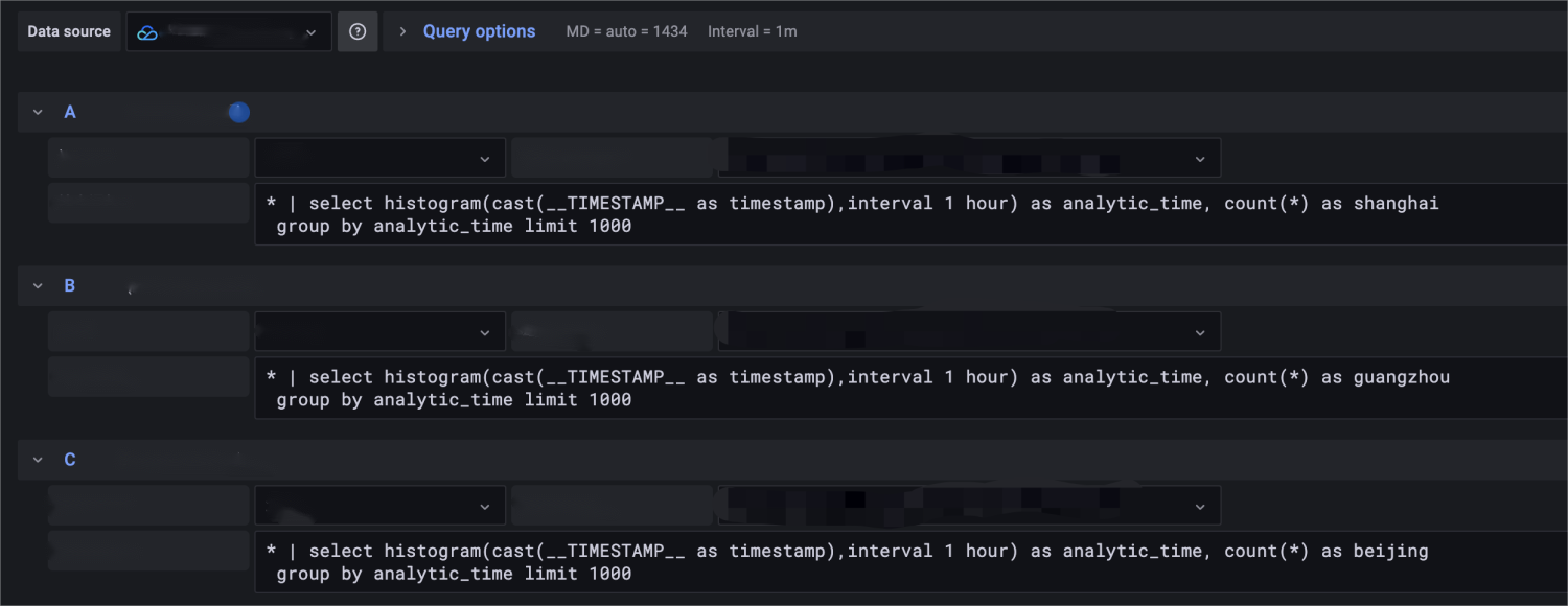
For three statements querying logs from different regions:
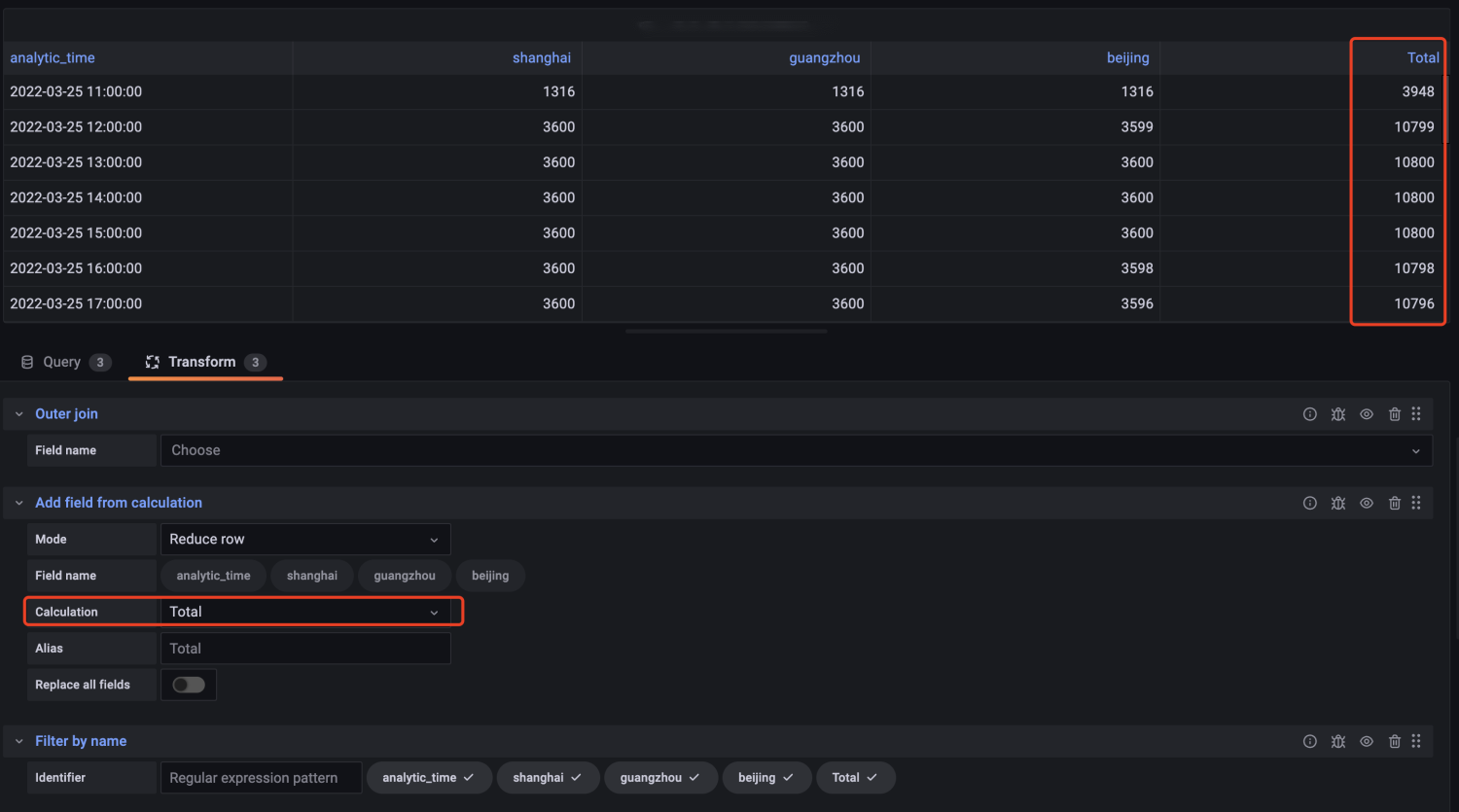
You can calculate the total numbers in the Transform module and select an appropriate chart to display them.
For three log queries from different regions:
We can use the Transform module to achieve the effect of data summation and select the required charts for display.
Summary
For existing ES dashboards, you can completely convert a dashboard with an ES data source into one with a CLS data source by repeating the migration steps described above. Migrating from ES to CLS data sources allows users to continue leveraging their accumulated visualization resources after users migrate from a self-built ELK stack to Tencent Cloud CLS. The converted dashboards not only fully match the capabilities of the ES data source version but can also integrate with the Tencent Cloud ecosystem more effectively by leveraging other features of the data source plugin, such as TCOP template variables.